EDA

Getting Start

In the code chunk below, p_load() of pacman package is used to load the R packages into R environemnt.

Show the code

pacman::p_load(igraph, tidygraph, ggraph, 
               visNetwork, lubridate, clock,
               tidyverse, graphlayouts, 
               concaveman, ggforce, jsonlite, dplyr, SmartEDA, knitr,scales,kableExtra,ggthemr)

# Import Data
kg <- fromJSON("data/MC1_graph.json")

Inspect Structure

In the code chunk below str() is used to reveal the structure of kg object.

Show the code

str(kg, max.level = 1)

List of 5
 $ directed  : logi TRUE
 $ multigraph: logi TRUE
 $ graph     :List of 2
 $ nodes     :'data.frame': 17412 obs. of  10 variables:
 $ links     :'data.frame': 37857 obs. of  4 variables:

Show the code

#Extracting the edges and nodes tables
nodes_tbl <- as_tibble(kg$nodes)
edges_tbl <- as_tibble(kg$links)

Creating Knowledge Graph

Before we can go ahead to build the tidygraph object, it is important for us to ensures each id from the node list is mapped to the correct row number. This requirement can be achive by using the code chunk below.

Show the code

#Mapping from node id to row index
id_map <- tibble(id = nodes_tbl$id,
                 index = seq_len(
                   nrow(nodes_tbl)))


#Map source and target IDs to row indices
edges_tbl <- edges_tbl %>%
  left_join(id_map, by = c("source" = "id")) %>%
  rename(from = index) %>%
  left_join(id_map, by = c("target" = "id")) %>%
  rename(to = index)


#Filter out any unmatched (invalid) edges
edges_tbl <- edges_tbl %>%
  filter(!is.na(from), !is.na(to))

#Creating tidygraph
graph <- tbl_graph(nodes = nodes_tbl, 
                   edges = edges_tbl, 
                   directed = kg$directed)

class(graph)

[1] "tbl_graph" "igraph"

Visualising the knowledge graph

In this section, we will use ggraph’s functions to visualise and analyse the graph object.

Several of the ggraph layouts involve randomisation. In order to ensure reproducibility, it is necessary to set the seed value before plotting by using the code chunk below.

Show the code

set.seed(1234)

Visualising the whole graph

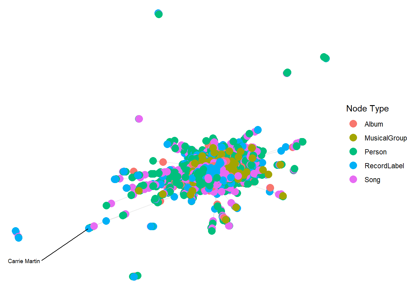
In the code chunk below, ggraph functions are used to visualise the whole graph.

Show the code

ggraph(graph, layout = "fr") +
  geom_edge_link(alpha = 0.3, 
                 colour = "gray") +
  geom_node_point(aes(color = `Node Type`), 
                  size = 4) +
  geom_node_text(aes(label = name), 
                 repel = TRUE, 
                 size = 2.5) +
  theme_void()

Warning: ggrepel: 17411 unlabeled data points (too many overlaps). Consider
increasing max.overlaps

Notice that the whole graph is very messy and we can hardy discover any useful patterns. In order to gain meaningful visual discovery, it is always useful for us to looking into the details, for example by plotting sub-graphs.

Visualizing Edge Types Frequency

ggplot(data = edges_tbl,
       aes(y = `Edge Type`)) +
  geom_bar()

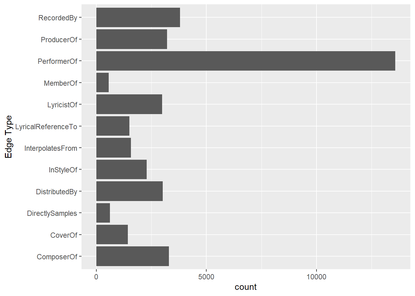
This bar chart above shows the distribution of different edge types in the music relationship network. The most common type is PerformerOf, indicating that the data heavily captures who performed which work. Other frequent types include ComposerOf, LyricistOf, and ProducerOf, highlighting the importance of creative and production roles. In contrast, relationships like MemberOf and DirectlySamples are less common, suggesting these connections are either rarer or less documented.

Visualizing Node Types Frequency

ggplot(data = nodes_tbl,
       aes(y = `Node Type`)) +
  geom_bar()

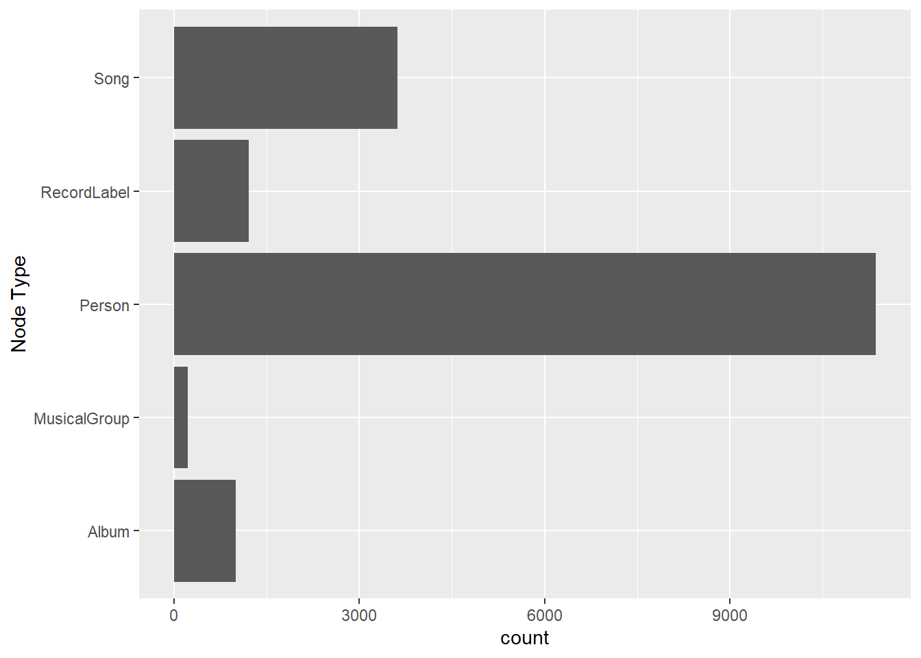
This bar chart displays the distribution of different node types in the music network dataset. The most common type is Person, with a count far exceeding other categories, indicating a strong focus on individual artists, producers, and contributors. Songs also appear in large numbers, highlighting the dataset’s emphasis on works being created or performed. Other types like Albums, RecordLabels, and MusicalGroups are present but in significantly smaller quantities.

Key Performance Indicators of Artists

Show the code

# Extract PerformerOf edge
graph_performers <- graph %>%
  activate(edges) %>%
  filter(`Edge Type` == "PerformerOf")

# Extract Performer nodes & works information
artist_influence <- graph_performers %>%
  activate(edges) %>%
  as_tibble() %>%
  left_join(nodes_tbl %>% select(id, name, `Node Type`, genre, notable, release_date, notoriety_date),
            by = c("target" = "id")) %>%
  rename(work_id = target,
         artist_id = source,
         work_name = name,
         work_type = `Node Type`) %>%
  left_join(nodes_tbl %>% select(id, name, stage_name), 
            by = c("artist_id" = "id")) %>%
  rename(artist_name = name) %>%
  filter(work_type %in% c("Song", "Album"),
         notable == TRUE) %>%
  select(artist_id, artist_name, stage_name, work_id, work_name, work_type, genre, 
         release_date, notoriety_date, notable)

# Export as CSV
write_csv(artist_influence, "artist_influence.csv")

#Convert "release_date" & "notoriety_date" as integer

influence <- artist_influence %>%
  mutate(
    release_year = as.integer(release_date),
    notoriety_year = as.integer(notoriety_date),
    is_notable = if_else(is.na(notoriety_date), FALSE, TRUE)
  )

Show the code

# Step 1: Summarise artist performance metrics
artist_summary <- influence %>%
  group_by(artist_name) %>%
  summarise(
    total_works = n(),
    years_active = n_distinct(release_year),
    first_notoriety = if (all(is.na(notoriety_year))) NA_integer_ else min(notoriety_year, na.rm = TRUE),
    notable_works = sum(is_notable),
    notable_years = n_distinct(notoriety_year[!is.na(notoriety_year)])
  ) %>%
  ungroup() %>%
  mutate(
    avg_works_per_year = round(total_works / years_active, 1),
    rising_star_score = notable_works * 2 + total_works + notable_years * 1.5
  ) %>%
  arrange(desc(rising_star_score))

# Step 2: Display the top 10 rising stars in a formatted table
artist_summary %>%
  slice_head(n = 10) %>%
  kbl(
    caption = "Table 1. Top 10 Rising Stars",
    col.names = c("Artist Name", "Total Works", "Years Active", "First Chart Year",
                  "Notable Works", "Notable Years", "Avg. Works/Year", "Rising Star Score"),
    align = "c"
  ) %>%
  kable_styling(
    bootstrap_options = c("striped", "hover", "condensed"),
    full_width = FALSE,
    position = "center"
  ) %>%
  row_spec(0, bold = TRUE, background = "#f2f2f2")

Table 1. Top 10 Rising Stars
Artist Name	Total Works	Years Active	First Chart Year	Notable Works	Notable Years	Avg. Works/Year	Rising Star Score
Kimberly Snyder	20	11	2023	5	2	1.8	33.0
Ping Tian	21	16	2010	3	3	1.3	31.5
Yang Zhao	18	8	2004	4	3	2.2	30.5
Qiang Tang	15	9	2010	4	4	1.7	29.0
Urszula Stochmal	15	11	2004	4	4	1.4	29.0
Lei Duan	14	10	1991	4	4	1.4	28.0
Ping Meng	14	11	2011	4	4	1.3	28.0
Szymon Pyć	20	14	2010	2	2	1.4	27.0
Gang Chen	9	8	2013	5	5	1.1	26.5
Jay Walters	16	15	1992	3	3	1.1	26.5

This table summarizes key performance metrics for each artist, including Total Works, Years Active, First Chart Year, Notable Works, Notable Years, and Average Works per Year.

To identify emerging talents, we calculate a composite Rising Star Score using the following formula:

Rising Star Score = 2 × (Notable Works) + (Total Works) + 1.5 × (Notable Years)

This scoring system gives additional weight to artists who consistently produce notable works and maintain visibility over multiple years, while also accounting for their overall productivity.

The table above lists the Top 10 artists with the highest Rising Star Scores, highlighting those who show strong potential and rising influence in the Oceanus Folk community.

Number of Songs and Album by Genre

Code

# Count the number of Songs and Albums in each genre
genre_summary <- nodes_tbl %>%
  filter(`Node Type` %in% c("Song", "Album")) %>%
  count(genre, `Node Type`) %>%
  pivot_wider(names_from = `Node Type`, values_from = n, values_fill = 0) %>%
  arrange(desc(Song + Album))


print(genre_summary)

# A tibble: 26 × 3
   genre                Album  Song
   <chr>                <int> <int>
 1 Dream Pop              152   590
 2 Indie Folk             108   342
 3 Synthwave               74   308
 4 Doom Metal              80   268
 5 Oceanus Folk            70   235
 6 Alternative Rock        53   205
 7 Southern Gothic Rock    57   185
 8 Indie Rock              52   156
 9 Americana               39   145
10 Psychedelic Rock        32   140
# ℹ 16 more rows

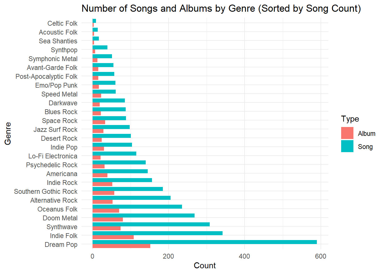
There are 26 unique genre in total in the network. Dream Pop have greates amount of release in terms of both song and albums among all genres. Dream pop have almost twice as many songs as the second genre(Indie Folk) do.

#| code-fold: true
#| warning: false
#| message: false

# 1. Sort by song count
genre_order <- genre_summary %>%
  arrange(desc(Song)) %>%
  pull(genre)

# 2. transform to long table
genre_long <- genre_summary %>%
  pivot_longer(cols = c(Song, Album), names_to = "Type", values_to = "Count") %>%
  mutate(genre = factor(genre, levels = genre_order))

# 3. plot the chart
ggplot(genre_long, aes(x = genre, y = Count, fill = Type)) +
  geom_bar(stat = "identity", position = position_dodge(width = 0.9)) +
  #geom_text(aes(label = Count),
            #position = position_dodge(width = 0.9),
            #hjust = 1.05, color = "black", size = 3.2) +
  labs(
    title = "Number of Songs and Albums by Genre (Sorted by Song Count)",
    x = "Genre",
    y = "Count"
  ) +
  theme_minimal() +
  coord_flip()

Dream Pop and Indie Folk have the most songs overall. In most genres, there are more songs than albums. Oceanus Folk is somewhere in the middle, with a fair number of both songs and albums. Some genres, like Celtic Folk and Sea Shanties, have very few works. This suggests that a few genres are very active, while many others are less popular or more niche

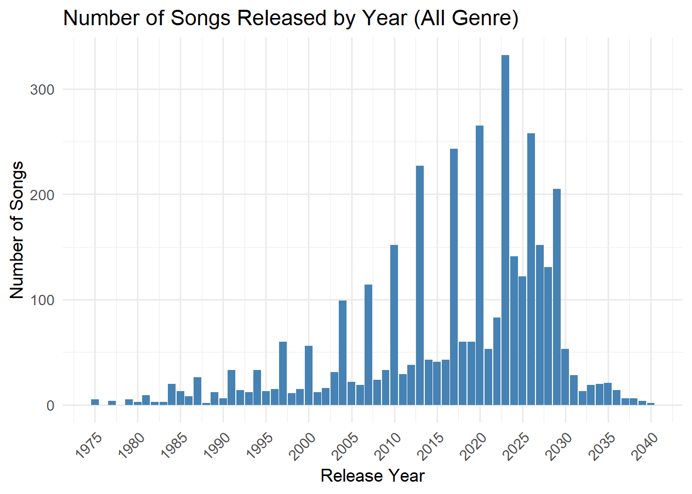
Number of Song Release by Year

Code

# Step 1: Filter song nodes with valid release date
songs_by_year <- nodes_tbl %>%
  filter(`Node Type` == "Song", !is.na(release_date)) %>%
  count(release_date, name = "count") %>%
  mutate(release_date = as.numeric(release_date))  # ⬅️ 确保为 numeric 类型

# Step 2: Plot chart with readable x-axis
ggplot(songs_by_year, aes(x = release_date, y = count)) +
  geom_col(fill = "steelblue") +
  scale_x_continuous(
    breaks = seq(min(songs_by_year$release_date, na.rm = TRUE),
                 max(songs_by_year$release_date, na.rm = TRUE),
                 by = 5)
  ) +
  labs(
    title = "Number of Songs Released by Year (All Genre)",
    x = "Release Year",
    y = "Number of Songs"
  ) +
  theme_minimal(base_size = 13) +
  theme(axis.text.x = element_text(angle = 45, hjust = 1))

The dataset covers song releases from 1975 to 2040. In general, the number of releases increased steadily from 1975, peaking around 2023. After that, the trend declines and returns to levels similar to those in the 1990s.

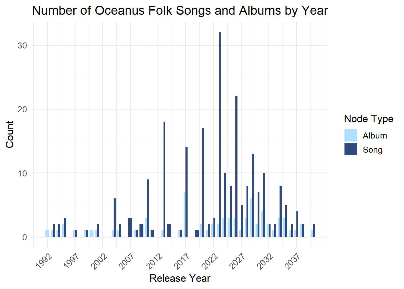
Number of Song and Album Release in Oceanus Folk Genre by Year

Code

# Step 1: Filter Oceanus Folk Songs and Albums with release date
oceanus_by_year <- nodes_tbl %>%
  filter(genre == "Oceanus Folk",
         `Node Type` %in% c("Song", "Album"),
         !is.na(release_date)) %>%
  count(release_date, `Node Type`, name = "count") %>%
  mutate(release_date = as.numeric(release_date))  # ⬅️ 转换为数值型

# Step 2: Plot chart with dodged bars
ggplot(oceanus_by_year, aes(x = release_date, y = count, fill = `Node Type`)) +
  geom_col(position = "dodge", width = 0.7) +
  scale_x_continuous(
    breaks = seq(min(oceanus_by_year$release_date, na.rm = TRUE),
                 max(oceanus_by_year$release_date, na.rm = TRUE),
                 by = 5)
  ) +
  labs(
    title = "Number of Oceanus Folk Songs and Albums by Year",
    x = "Release Year",
    y = "Count"
  ) +
  scale_fill_manual(values = c("Song" = "#2f4b7c", "Album" = "#b2defd")) +
  theme_minimal(base_size = 13) +
  theme(axis.text.x = element_text(angle = 45, hjust = 1))

This chart shows the number of Oceanus Folk songs and albums released by year. The number of releases gradually increased from the early 2000s and peaked around 2023.Most of the releases are songs, while albums remain fewer across all years. After 2023, there is a slight decline, but both songs and albums continue to be released steadily until the late 2030s. Before 2010, Oceanus Folk activity was very limited. This suggests that Oceanus Folk started gaining popularity in the 2010s and became most active in the early 2020s.